Most people consider the Fundamental Theorem of Calculus the crown jewel of single variable calculus. It’s hard to argue with them; the theorem captures the essence of calculus by marrying differentiation and integration in a (relatively) simple statement. However, I find that it’s at differential equations and modelling where the ideas and tools of calculus really begin to shine and students’ appreciation for the subject reaches its maximum. (Pun very much intended.) Therefore I think it important to let students see not only the wonderful theory of (ordinary) differential equations, but also their predictive power. And by ‘seeing’ I mean really experiencing how a simple ODE can in fact model Nature.

To achieve this, I came up with a couple of practical demonstrations that anyone can perform and use to impress upon students just how awesome calculus is. During the past four years, the demos have been tested in the classroom and the student response has been overwhelmingly positive. Here are my criteria for effectiveness: the demos must be T1) instructive, T2) short (<10 mins), T3) cheap (< €10), T4) easy to implement (very little to no skill is required). From the student perspective, an ideal demo is S1) relevant, S2) simple to understand, yet S3) illuminating, and S4) fun!

The first demonstration I’m going to share with you is called “Calculus is COOL”. It’s about Newton’s Law of Cooling, a harmless first-order linear ODE, which, despite its simplicity, highlights the importance of assumptions in model building, initial values, model parameters, margins of error, etc. All you need is a mug of warm water and a thermometer (see figure 1). If your classroom has a PC and projector (as most does), you may use a smartphone and a digital thermometer (with Bluetooth connection) to project the temperature readings. I also use a really nice calculator app to do live computations on the big screen. (Alternatively, you may simply cast the picture of your phone camera aimed at the thermometer.) The links to the various apps used for this activity are included below.

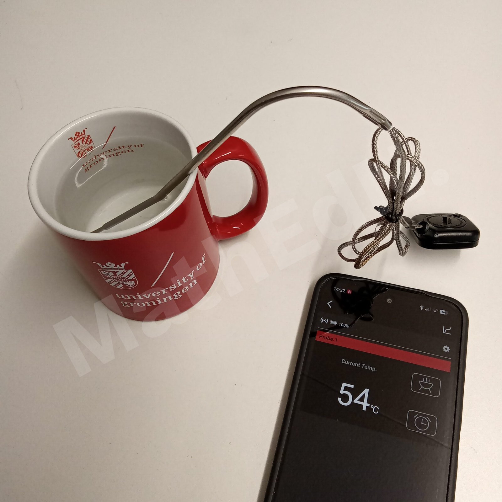
[FIGURE 1: The setup is super basic: a mug of hot water and a thermometer.]

For context, this demonstration takes place in the last 10 minutes of the first lecture we have on differential equations. During the lecture, we cover the basics: what’s an ordinary differential equation, independent and dependent variables, order, direction field, solution curves, initial value problems, separable & linear ODEs, etc. We set up and solve the standard examples of natural growth, radioactive decay, and mixing throughout the lecture. Then, as we approach the end of the lecture, I tell the students that they have absolutely no reason to believe me when I say that this stuff – modelling with ODEs – works. After all, there is nothing to guarantee that Nature obeys such neat and orderly mathematics. So I propose that we test it right there and then. I go and fetch some hot water from a nearby coffee machine, note down the ambient (room) temperature, dip the thermometer in and set a timer for 10 minutes. Then I make the bold claim that we are about to predict the future, that is the temperature of hot water 10 minutes from now. What follows is a quick back and forth where I ask students how they think hot objects cool down. It only takes a minute for them to come up with a model: the rate of change of the temperature of an object is proportional to the temperature difference between the environment and the object. This is exactly Newton’s law of cooling! We formulate it as an ODE

T'(t)=r[Tₑₙᵥ-T(t)].

Here r is a constant (the coefficient of heat transfer) and Tₑₙᵥ is the temperature of the environment (also assumed to be constant). By solving the initial-value problem using separation of variables we obtain the general solution

(*) T(t)=Tₑₙᵥ+(T₀−Tₑₙᵥ)exp(-rt),

where T₀=T(0) is the initial temperature of the object. Looking at the solution, we do a quick sanity check: at t=0 we have indeed T(0)=T₀ and as time goes to infinity we approach the ambient temperature. Then we record the value of T₀ and Tₑₙᵥ, but at this point (around 5 minutes into the experiment), we realize that the value of the parameter r is missing. Thus we have to make a measurement. To give you some actual numbers from a previous run, we had Tₑₙᵥ = 21.5∘C, T₀ = 54∘C and after 5 minutes we measured T₅ = 51∘C. (For dramatic effect, I hide the live temperature reading at this point and only reveal it when the 10 minutes are up.) We use these data and compare it to the solution in equation (*) (evaluated at t=5) to find a value for r:

r = (1/5) ln[(T₀−Tₑₙᵥ)/(T₅−Tₑₙᵥ)] ≈ 0.02208

Thus we are able to predict the temperature at t=10 (minutes):

T(10) = Tₑₙᵥ+(T₀−Tₑₙᵥ)exp(−10r) ≈ 44.3∘C

By the time we reach this point the timer is almost up and the students are super exited to see whether our prediction is correct. I remind them that my cheap thermometer can only measure temperature in integer units so we round down and predict the final temperature to be 44∘C. As the timer goes off, I make the big reveal and our (rather primitive) thermometer reads T₁₀ = 44∘C. The room breaks out in applause. I tell them that we also had some luck and that sometimes the prediction is off by 1 degree due to the crude measurements and propagation of error.

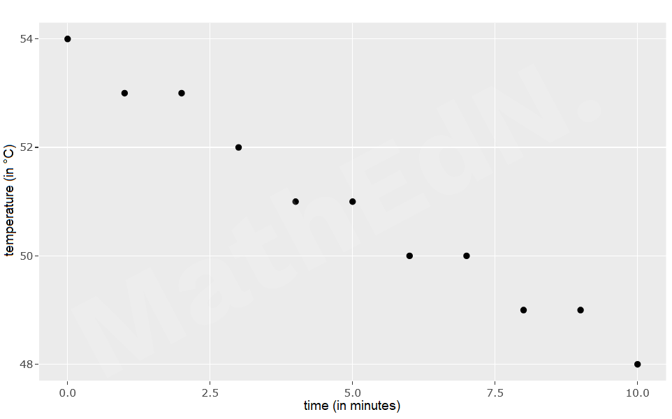
[FIGURE 2: Data from the 10-minute experiment we did during the lecture]

After the lecture, I share the data from a 90-minute experiment (with Tenv=20.5∘C, T0=78∘C, T10=63∘C) I’ve done the day before (see figure 3) and I ask them the following questions:

1. What is the value of the coefficient r in Experiment 2?

2. How good is the prediction of the solution T(t) for the measured temperatures T20, T40, T60, T80?

3. Fit a function of the form T∗env+(T0−T∗env)e−r∗t to the data using the data points T0, T10, T20, T30. What values does your fit assign to T∗env and r∗? Are these value close to Tenv and r?

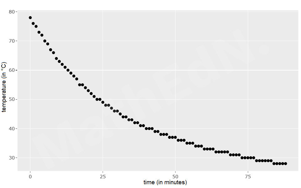
[FIGURE 3: Data from the 90-minute experiment from the day before the lecture.]

Finally, I put up a challenge to solve a related problem: Suppose you have a cup of hot coffee and some cream at room temperature. You need to go make a phone call for 5 minutes. Should you mix in the cream before or after the call to ensure your coffee stays as hot as possible?

I hope you find this demonstration inspiring. If you decided to try it out with your students, feel free to get in touch, I’d love to know how it went. Have fun!

Apps:

Screen Stream app to cast phone screen (https://play.google.com/store/apps/details?id=info.dvkr.screenstream&hl=en)

Calculator app (https://play.google.com/store/apps/details?id=uk.co.nickfines.RealCalc&hl=en)

Thermometer app with built in timer (https://play.google.com/store/apps/details?id=com.togrill.haibosi&hl=en)

Links:

Calculus is COOL. https://tamasgorbe.com/calculus

The coffee and cream challenge. Matt Parker explains and demonstrates what will happen: https://www.youtube.com/watch?v=CCuaWqhVvIc [SPOILER ALERT]